Detecting Opps (Opponents in Autonomous Vehicles Race)

Our team is working to incorporate computer vision as an object tracking modality. We’re using a YOLOv5 model to do this, and the most difficult part has been to collect data. We use a semi-automated pipeline to achieve a high quantity of data through auto-labeling, without sacrificing on quantity.

Context: Object Detection for Autonomous Racing

Our autonomous vehicle is supplied by the Indy Autonomous Challenge, which includes several state-of-the-art Luminar LiDAR sensors as well as six cameras (two front-facing, normal FOV cameras, and four wide-angle to capture the side and back views).

Each camera sends detections to a YOLOv5 model, which provides bounding boxes for the opponent vehicle. When given bounding boxes for the opponent that correspond across multiple views, we can calculate a 3D position. Because all cars used in this race have the same dimensions (the frames are provided by Dallara, an Italian auto manufacturer), we can use the size of the vehicle to estimate depth.

To calculate the direction, we can use our knowledge of the camera’s intrinsic/extrinsic matrices and distortion parameters. The cameras on this car follow a Brown-Conrady distortion model, and although I have no idea how to derive how that works, I do know that I can use OpenCV to undistort the images for me! So I just use that, along with the distortion parameters provided from the manufacturer. We can calculate the direction of the opponent vehicle in map frame by taking the undistorted 2D locations on the camera’s embedding plan (at \(z = 1\)) and then rotating them to map frame. Given a point \([x, y, 1]\) on the camera embedding plane, we can undistort this to world frame simply by applying the camera’s rotation matrix \(R\) (more information in the Camera Background: Pinhole Camera Model section below). Then, we can scale this by the estimated depth of the vehicle, and add the camera’s translation vector \(\hat t = (x, y, z)\) to get the final 3D position in map frame.

We train these models using the standard pipeline from Ultralytics. We provide 2D bounding box labels for a large dataset of images collected from real-life historical data: an MIT-KAIST race from LVMS in a prior year, a UVA-MIT race from LVMS 2024, and a Euroracing-TUM race.

We are using Grounding Dino to generate labels. This is a great foundation model, although we cannot use it in the race for two reasons: (1) it is slow; (2) there are some false positives (e.g. non-Indy cars). YOLO (or similar) models provide an opportunity to create distilled versions of foundation models with the added benefits of high speed and a more curated dataset.

We have a simple method for eliminating false positives from human supervision. We iterate through the video, frame-by-frame, automatically labelling new bounding boxes as correct if they are within a certain pixel distance of the previous detection. However, when a false positive appears, it is generally a high distance from our current car detection, and we automatically discard those. Whenever there is ambiguity (for example, the opponent enters the frame, and we cannot determine whether the label is accurate or not automatically), we defer to human supervision. This does not happen often. The end result is that we can take advantage of the general capability of the foundation model to detect cars, while simultaneously curating with human feedback.

Result

The resulting model is \(14\) Mb, which is great and can run at high Hz. Additionally, it has significantly higher recall than the original foundation model. We have integrated this into our object detection pipeline, and using the simple monocular depth estimation equation from before, we can estimate 3D location: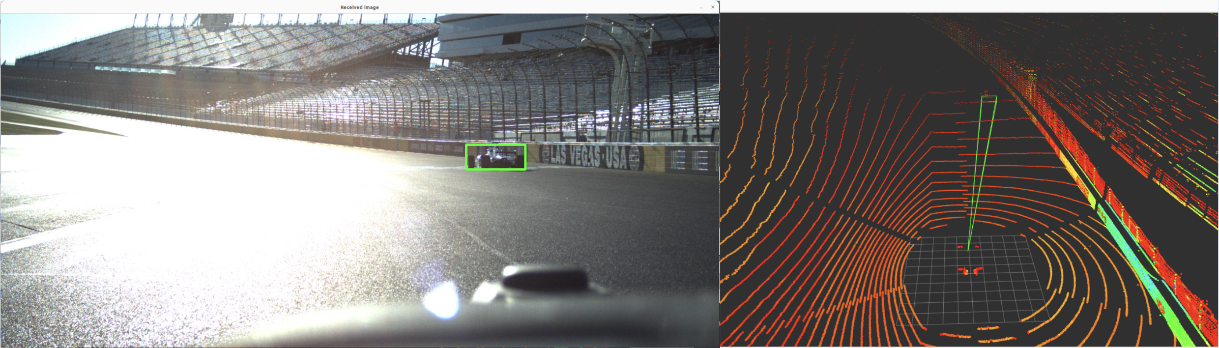

Additionally, we find that the resulting model is excellent even in harsh lighting conditions. The following image grid consists only of images that were not in the training dataset, because their labels were not detected successfully by the foundation model: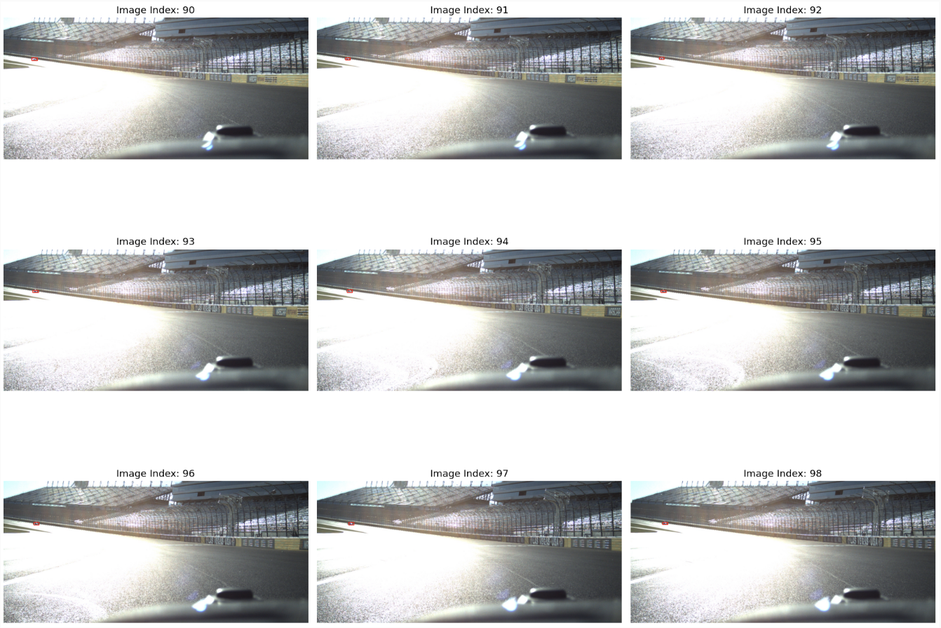

Camera Background: Pinhole Camera Model

Feel free to skip this section if you already know how the pinhole camera model works!

Cameras are determined by a position/orientation (extrinsic) and a focal length (intrinsic). Intrinsic means no matter how you move the camera around, they will stay the same. Extrinsic means when you move the camera, they change.

The pinhole camera model maps 3D locations to images. This is done via matrix multiplication. Think of matrix multiplication as rotating the world. We rotate the world so that (0, 0, -1) faces the camera. Then x and y in this rotated world correspond to the same x and y directions as an image. We use the intrinsic matrix to convert x and y in these rotated coordinates into pixel values (e.g. 1 meter in world coordinates becomes, say, 240 pixels). There is also a notion of translation; just think of this as subtracting coordinates so that (0, 0, 0) in the translated world is at the center of the camera.

Extrinsics

An extrinsic camera matrix follows the following format: [R t] where R is a 3x3 rotation matrix and t is a 3x1 translation vector.

The extrinsic matrix is something that takes a point in rear_axle_middle_ground frame and converts it to “camera” frame. The main difference between these (besides the angle/perspective of the camera) is the difference between the axes.

For the car, “forward” is X, “right” is Y, and “up” is Z. For the camera, though, “forward” is Z, “right” is X, and “up” is Y (or -Y, if you go top->bottom in images).

Let’s say we want to design a matrix to convert a point in “world coordinates” to the coordinates from the point of view of the camera.

The first step is to translate. Let’s say the input point is (x, y, z), and the camera’s location is (tx, ty, tz). We can write this as a (4D) matrix multiplication in the following way:

[1 0 0 -tx][x]   [x - tx]
[0 1 0 -ty][y] = [y - ty]
[0 0 1 -tz][z]   [z - tz]
[0 0 0   1][1]   [1     ]

Consider this from the perspective of the camera. A point at (tx, ty, tz) must go to the point (0, 0, 0) from the perspective of the camera. So this is the first part.

translation = np.array([
    [1, 0, 0, -x],
    [0, 1, 0, -y],
    [0, 0, 1, -z],
    [0, 0, 0, 1],
])

The next step is to rotate. Imagine the camera is pointing straight ahead.

For a rotation matrix (which is orthonormal), every row represents what that part of the matrix is “detecting”. To explain more clearly, consider this matrix:

    [0 1 0 0][x]   [y]
    [0 0 1 0][y] = [z]
    [1 0 0 0][z]   [x]
    [0 0 0 1][1]   [1]

Recall: For the car, “forward” is X, “right” is Y, and “up” is Z. For the camera, though, “forward” is Z, “right” is X, and “up” is Y (or -Y, if you go top->bottom in images).

This means that for the output of this matrix,

• Row 1 (the “x” row) is detecting Y values, by dot-producting [0 1 0 0] with [x y z 1]
• Row 2 (the “y” row) is detecting Z values, by dot-producting [0 0 1 0] with [x y z 1]
• Row 3 (the “z” row) is detecting Z values, by dot-producting [1 0 0 0] with [x y z 1]

This makes sense if you consider a matrix multiplication onto a vector as dotting each row of the matrix with the vector to produce a new vector.

Another thing this means is that if we invert the rotation matrix (which, by virtue of being orthonormal, amounts to a matrix transpose [making the rows -> columns and vice versa]), then multiplying by a point in “camera” coordinates outputs how the point would look in rear_axle_middle_ground coordinates.

To create the final camera extrinsics matrix, we multiply the rotation matrix by the translation matrix. This creates a matrix that has the same effect of (1) translating the world to the center of the camera, and (2) rotates the world so the coordinate axes line up with the axes of the image.