
Sparse Autoencoder
Published:
What kinds of useful features can we extract from images?
I wonder how we can meaningfully code for orientation and scale in images through neural networks. My goal is to maximize the number of explainable features that neural networks generate.
I experiment with the CelebA dataset and finetune a pretrained model (from ImageNet) to disambiguate between faces. The goal is that the model learns to output a fine-tuned vector space that distinguishes between faces. I could use a VAE but that takes a while; instead I will estimate mean and variance from a decent batch size and use KL divergence on that.
Download Dataset
We’ll be using the CelebA dataset for this. I’ll assume you have a Kaggle account and can download with that. To save me from the hassle of kaggle.json, I’m using environment variables.
# First, download CelebA dataset.
import os
import getpass

os.environ['KAGGLE_USERNAME'] = getpass.getpass("Username")
os.environ['KAGGLE_KEY'] = getpass.getpass("API Key")

!kaggle datasets download -d jessicali9530/celeba-dataset -p CelebA
Username··········
API Key··········
Downloading celeba-dataset.zip to CelebA
100% 1.33G/1.33G [00:12<00:00, 230MB/s]
100% 1.33G/1.33G [00:12<00:00, 117MB/s]
# Our images unzip to `./img_align_celeba/img_align_celeba` (relative to the current directory; not the CelebA folder for some reason.)
!unzip CelebA/celeba-dataset.zip -d data > /dev/null
Load dataset
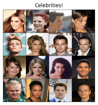
Loading images from a folder is a common process, so Torchvision has a way for us to do this automatically. To test that everything works, I set up a quick visualization. It renders the first 16 images as a 4x4 grid using matplotlib.
import matplotlib.pyplot as plt
import torch
import torchvision
import torchvision.transforms as T
from torch.utils.data import DataLoader
from torchvision.datasets import ImageFolder

def visualize_4x4(images: torch.Tensor, title=None):
    # Shape: [N, C, H, W]

    # Make a grid of images
    grid = torchvision.utils.make_grid(images, nrow=4).numpy()

    # Render
    plt.figure(figsize=(4, 4))
    plt.title(title or "Celebrities!")
    plt.imshow(grid.transpose((1, 2, 0)))
    plt.axis("off")
    plt.show()

# Now, train a contrastive model. Use CelebA dataset.
# dataset[i] = (PIL.Image.Image, <dummy class label>)
dataset = ImageFolder(root="./data", transform=T.Compose([
    T.ToTensor(),
    T.Resize((224, 224)),
]))

visualize_4x4([dataset[i][0] for i in range(16)])
/usr/local/lib/python3.10/dist-packages/torchvision/transforms/functional.py:1603: UserWarning: The default value of the antialias parameter of all the resizing transforms (Resize(), RandomResizedCrop(), etc.) will change from None to True in v0.17, in order to be consistent across the PIL and Tensor backends. To suppress this warning, directly pass antialias=True (recommended, future default), antialias=None (current default, which means False for Tensors and True for PIL), or antialias=False (only works on Tensors - PIL will still use antialiasing). This also applies if you are using the inference transforms from the models weights: update the call to weights.transforms(antialias=True).
  warnings.warn(
Training
We’ll use a resnet18 pretrained model which is pretty standard, and it should have decent feature representations already, which should easily be finetuned to this domain.
from torchvision.models import resnet

# Decide whether to use the GPU. This speeds up training a *LOT* if it's available.
device = torch.device('cuda' if torch.cuda.is_available() else 'cpu')

model = torch.hub.load('pytorch/vision:v0.10.0', 'resnet18', pretrained=True)
# Remove the fully-connected layer because we're interested in embeddings.
model.fc = torch.nn.Identity()
model = model.to(device)
Using cache found in /root/.cache/torch/hub/pytorch_vision_v0.10.0
/usr/local/lib/python3.10/dist-packages/torchvision/models/_utils.py:208: UserWarning: The parameter 'pretrained' is deprecated since 0.13 and may be removed in the future, please use 'weights' instead.
  warnings.warn(
/usr/local/lib/python3.10/dist-packages/torchvision/models/_utils.py:223: UserWarning: Arguments other than a weight enum or `None` for 'weights' are deprecated since 0.13 and may be removed in the future. The current behavior is equivalent to passing `weights=ResNet18_Weights.IMAGENET1K_V1`. You can also use `weights=ResNet18_Weights.DEFAULT` to get the most up-to-date weights.
  warnings.warn(msg)
Training the model
Because this is a smaller model, its capacity is strained for distinguishing between faces. This model was trained to detect objects of a certain range of classes (in ImageNet), and its internal/latent representation is a continuous vector. Classifications are made by having class-specific vectors that are dotted with the latent vector to create scores. In this case, we want to minimize the similarity between vectors belonging to different faces; so we use a contrastive loss. This forces the model to output dissimilar vectors for dissimilar faces. By inspecting the mapping the model creates as a result (which we assume will create similar vectors for similar faces, as the model is forced to compress some of the information it sees), we can try to extract salient facial features.
The loss function is as follows. Let $X$ be the set of input images. \(y \leftarrow \text{Model}(X) \\ \text{Loss}(y) := L_{ce} + L_{orient}\)
Where Cross Entropy is defined as \(L_{ce}(logprobs, target) := -\sum_{i=0}^{k} target_i logprobs_i\)
Where $logprobs$ is the log-Softmax output of the prediction vector.
To train the model to incorporate implicit orientation, I train it to reduce the mean-squared-error between the encoding of the input image and the negative of the encoding of the flipped image. \(L_{orient}(y_{normal}, y_{flipped}) := L_{mse}(y_{normal}, -y_{flipped})\)
import tqdm

batch_size = 128
dataloader = DataLoader(dataset, batch_size=batch_size, shuffle=True)

optim = torch.optim.Adam(model.parameters(), lr=1e-3)

N_EPOCHS = 1
for epoch in range(N_EPOCHS):
  with tqdm.tqdm(dataloader, desc="Training...") as pbar:
    for (images, _) in pbar:
      images = images.to(device)
      # Train model to disambiguate between these images.
      # Use embeddings as features. Instead of retraining
      # all of EfficientNet, add a linear layer at the end
      # to get embeddings. Rotate vector around first dimension.
      # 180º rotated images should have negative embeddings of each other.
      images_rotated = torch.rot90(images, 2, (2, 3))
      # [N, embedding_dim]
      embeddings = model(images)
      embeddings_rotated = model(images_rotated)

      # ORIENTATION LOSS
      loss_orientation = torch.nn.functional.mse_loss(embeddings, -embeddings_rotated)

      # CONTRASTIVE LOSS
      # Dot each of these embeddings with each other and treat these as logits.
      # Then use Cross Entropy loss.
      embeddings_normalized = torch.nn.functional.normalize(embeddings, dim=1)
      scores = embeddings @ embeddings.T
      loss_contrastive = torch.nn.functional.cross_entropy(scores, torch.arange(len(scores), device=device))

      loss = loss_contrastive + loss_orientation

      optim.zero_grad()
      loss.backward()
      optim.step()
      pbar.set_postfix({"loss": loss.item(), "contrastive_loss": loss_contrastive.item(), "orientation_loss": loss_orientation.item()})
Training...: 100%|██████████| 1583/1583 [34:38<00:00, 1.31s/it, loss=0.0944, contrastive_loss=0.00796, orientation_loss=0.0864]
Save our model.
This took like half an hour. I trained on the whole of CelebFace while writing the below content. Let’s please save this model lol.
torch.save(model.state_dict(), "resnet_18_celebface_state_dict.pt")
Create inferences.
We did a single pass over this dataset. Let’s create vectors for each of the faces in the dataset now.
results = []
model.eval()

# Notably, we *DO NOT SHUFFLE*!
dataloader_eval = DataLoader(dataset, batch_size=batch_size, shuffle=False)

with torch.no_grad():
  with tqdm.tqdm(dataloader_eval, desc="Generating output vectors...") as pbar:
    for (images, _) in pbar:
      images = images.to(device)
      embeddings = model(images)
      results.append(embeddings.to('cpu'))

# Took about 17m50s for 1583 batches (202599 input faces)
# Generate a single tensor
face_vectors = torch.cat(results, dim=0)

# See how much data we got :0
# Each vector has 512 dimensions.
print(face_vectors.shape)

# Store this tensor
torch.save(face_vectors, "face_vectors.pt")
torch.Size([202599, 512])
After training for a bit, we hopefully have a model that is strong at distinguishing different faces! (I only trained on 1/3 of the dataset, but it’s probably fine… the dataset is big and this is just for experiment.)
I want to see what the most salient features are for this model, too. How can we do this?
A page from Stanford CS231n shares a nice overview of ways to evaluate CNNs. One blog post shares a suite of ways to visualize convolutional neural network predictions. We can:
- Visualize maximally-activating patches (i.e., see what inputs for the receptive field of a given output cause the highest activation). We do this by inputting a bunch of images and see which ones are the most strongly correlated with certain features.
- Occlusion and gradient-based experiments are useful for identifying what contributed the most to an output. Examples include SHAP, GradCAM, and Integrated Gradients.
- We can look at the gradient of a classification w.r.t a specific part of the input image, or we can occlude parts of the image and see how our classification changes.
- Deconv/Guided backprop are ways to synthetically generate maximally-activating patches. Basically, we are causing the model to hallucinate a given response, and inspecting what input it’s “imagining”. One popular example is DeepDream. See Peeking Inside ConvNets for a page with nice examples.
- On a technical level, what we’re doing is using the same technique for optimizing model weights against a loss function to optimize an image input against a class activation. We start with an image and perform gradient descent, using the class activation as the objective (so $loss = -activation$).
- Embeddings: We can use methods like t-SNE to reduce the dimensionality of input images. Essentially, output vectors (which can be in a massive $512$-dimension vector space, etc.) are converted to 2D vectors, in a way that keeps neighboring vectors in the larger space close together in the 2D space. This gives a nice at-a-glance way to visualize what images the network perceives as similar to each other.
With respect to language models, Anthropic introduces a Sparse Autoencoder, which takes the set of output features (which form a densely-packed vector space of real-valued dimensions) and outputs a large set of disrete features. This is similar to work done by OpenAI to discover multimodal neurons.
- The sparse autoencoder is used specifically in language models. The goal of the sparse autoencoder is to discover features with monosemanticity. Because the inner workings of language models are not regularized at all, the intermediate vector space can look like a mess, as long as the optimizer knows how to improve predictions given more input. Although it makes optimization simply “work”, it’s bad for us because we don’t know what anything means. Additionally, because we can assume that most words don’t have all possible semantic meanings at once, some sort of compression is happening, resulting in an overpopulated basis. What this means is that $1024$ binary features might be stored in a $512$-dimensional real-valued vector. Why is this bad? Because we can’t point to any one feature and say, “this is the poetry detector”. What the sparse autoencoder does is take the range of internal representations the model creates across a wide variety of inputs, and translates it to a vector space where each dimension of the vector corresponds to a different feature.
I realized I forgot to store the output vectors of the model. It’s fine; using torch.no_grad() for non-training tasks makes compute take less time. Also, this is just for experimentation.
The question is now, will the model identify my face separately from someone elses? (And what features might the model be using?)
Testing Methods
We’ll now try various attribution methods to understand the features of our model. I’ll use the sparse autoencoder proposed by Anthropic for this. The method resembles a standard linear encoder and decoder, with the difference that decoder bias is subtracted from the input before being encoded. \(\overline{x} = x - b_d \\ f = \text{ReLU}(W_e\overline{x} + b_e) \\ \hat{x} = W_df+b_d \\ L = \frac{1}{|X|} \sum_{x \in X} \|x - \hat{x}\|_2^2 + \lambda\|\textbf{f}\|_1\)
The loss function $L$ decomposes into:
- A reconstruction loss (input vs. reconstructed input; MSE)
- A regularization loss (L1 norm of sparse features)
class SparseAutoencoder(torch.nn.Module):
  def __init__(self, input_feature_dim, sparse_feature_dim):
    super().__init__() # necessary for any torch.nn.Module subclass

    self.weight_encoder = torch.nn.Parameter(torch.zeros((input_feature_dim, sparse_feature_dim), dtype=torch.float32))
    self.weight_decoder = torch.nn.Parameter(torch.zeros((sparse_feature_dim, input_feature_dim), dtype=torch.float32))
    self.bias_decoder = torch.nn.Parameter(torch.zeros(input_feature_dim, dtype=torch.float32))
    self.bias_encoder = torch.nn.Parameter(torch.zeros(sparse_feature_dim, dtype=torch.float32))
    # initialize weight matrices
    torch.nn.init.normal_(self.weight_encoder)
    torch.nn.init.normal_(self.weight_decoder)

  def encode(self, input_features):
    # (n, input_feature_dim)
    xbar = input_features - self.bias_decoder
    # (n, sparse_feature_dim)
    f = torch.nn.functional.relu(xbar @ self.weight_encoder + self.bias_encoder)
    return f

  def decode(self, sparse_features):
    # (n, sparse_feature_dim)
    xhat = sparse_features @ self.weight_decoder + self.bias_decoder
    return xhat

def sparse_autoencoder_loss(model, input_features, l1_lambda):
  # Assume input is batched: (n, input_feature_dim)
  f = model.encode(input_features)
  x_hat = model.decode(f)
  # L_reconstruction = torch.nn.functional.mse_loss(input_features, x_hat)
  L_reconstruction = torch.norm(input_features - x_hat, 2)
  L_complexity = l1_lambda * torch.norm(f, 1)
  return L_reconstruction, L_complexity
Detecting Important Features
Here, we use the Sparse Autoencoder to detect monosemantic features. (I could have added an L1 loss to the feature vectors during training at minimal overhead…)
We first load the face vectors we saved. (My runtime crashed, lol.)
import PIL.Image
import torch

face_vectors = torch.load("face_vectors.pt")
sparse_feature_dim = 512
sae = SparseAutoencoder(input_feature_dim=512, sparse_feature_dim=sparse_feature_dim).to('cuda')
sae_optim = torch.optim.Adam(sae.parameters(), lr=1e-5, weight_decay=1e-4)
import tqdm

# l_recon = 30 or so.
# Takes like 1 minute train this many epochs, because of CUDA and the small size of the dataset.
for epoch in range(30):
  i = 0
  sae_batch_size = 512
  N = len(face_vectors)
  order = torch.randperm(N)
  with tqdm.tqdm(total=N, desc="Training sparse autoencoder...") as pbar:
    while i < N:
      batch = face_vectors[order[i:i + 512]].to('cuda')
      # L_reconstruction, L_complexity = sparse_autoencoder_loss(sae, torch.nn.functional.normalize(batch) * torch.sqrt(torch.tensor(512.0)), l1_lambda=0.1)
      L_reconstruction, L_complexity = sparse_autoencoder_loss(sae, torch.nn.functional.normalize(batch), l1_lambda=0.1)
      loss_sae = L_reconstruction + L_complexity
      sae_optim.zero_grad()
      loss_sae.backward()
      sae_optim.step()
      pbar.set_postfix({"loss_sae": loss_sae.item(), "recon": L_reconstruction.item(), "compl": L_complexity.item()})
      pbar.update(sae_batch_size)
      i += sae_batch_size
# Save our sparse autoencoder.
torch.save(sae.state_dict(), "sparse_autoencoder_weights.pt")
Generate features for each image
Now that we’re done training, let’s infer the feature set for each image.
# Let's sort images by their activation of certain neurons.
sparse_features = []

with torch.no_grad():
  i = 0
  sae_batch_size = 512
  N = len(face_vectors)
  with tqdm.tqdm(total=N, desc="Extracting sparse features...") as pbar:
    while i < N:
      batch = face_vectors[i:i + 512].to('cuda')
      sparse_features.append(sae.encode(batch).to('cpu'))
      i += sae_batch_size
      pbar.update(sae_batch_size)

feats = torch.cat(sparse_features, dim=0)
Extracting sparse features...: 202752it [00:00, 419656.01it/s]
# Save our sparse features.
torch.save(feats, "face_vectors_sparse.pt")
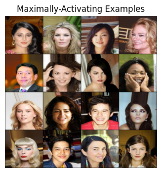
Inspecting Results
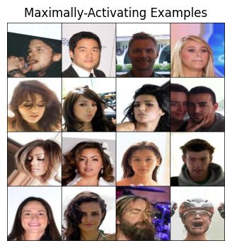
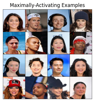
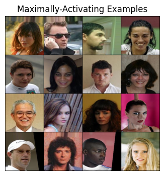
The sparse autoencoder has now been trained. Now, let’s look at which images maximally activate each feature. I’ll normalize the features using torch.nn.functional.normalize before sorting so we can look at which images have the strongest relative activation for each feature.
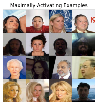
Result Without Sparse Autoencoder
Let’s see if the initial face vector (i.e., before being encoded) has interpretable feature representations.
feats_dense_normed = torch.nn.functional.normalize(face_vectors)

for feature_id in range(16):
  # Sort images by feature `feature_id`.
  order = torch.argsort(feats_dense_normed[:, feature_id], descending=True)
  visualize_4x4(
      [dataset[order[i]][0] for i in range(16)],
      title="Maximally-Activating Examples",
  )
/usr/local/lib/python3.10/dist-packages/torchvision/transforms/functional.py:1603: UserWarning: The default value of the antialias parameter of all the resizing transforms (Resize(), RandomResizedCrop(), etc.) will change from None to True in v0.17, in order to be consistent across the PIL and Tensor backends. To suppress this warning, directly pass antialias=True (recommended, future default), antialias=None (current default, which means False for Tensors and True for PIL), or antialias=False (only works on Tensors - PIL will still use antialiasing). This also applies if you are using the inference transforms from the models weights: update the call to weights.transforms(antialias=True).
  warnings.warn(
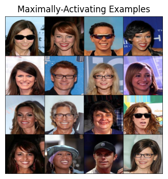
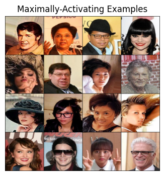
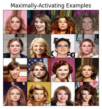
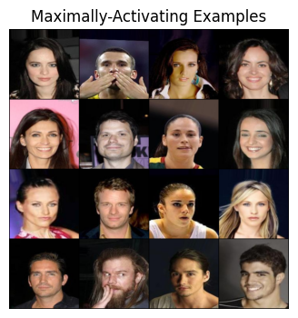
Result With Sparse Autoencoder
feats_normed = torch.nn.functional.normalize(feats)

for feature_id in range(16):
  # Sort images by feature `feature_id`.
  order = torch.argsort(feats_normed[:, feature_id], descending=True)
  visualize_4x4(
      [dataset[order[i]][0] for i in range(16)],
      title="Maximally-Activating Examples",
  )
/usr/local/lib/python3.10/dist-packages/torchvision/transforms/functional.py:1603: UserWarning: The default value of the antialias parameter of all the resizing transforms (Resize(), RandomResizedCrop(), etc.) will change from None to True in v0.17, in order to be consistent across the PIL and Tensor backends. To suppress this warning, directly pass antialias=True (recommended, future default), antialias=None (current default, which means False for Tensors and True for PIL), or antialias=False (only works on Tensors - PIL will still use antialiasing). This also applies if you are using the inference transforms from the models weights: update the call to weights.transforms(antialias=True).
  warnings.warn(
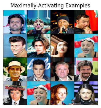
Unbiased Blind Interpretability Test
To see whether there is a measurable difference between the feature encoders, I’ll take a few features I haven’t seen before and rate each feature for its explainability. Then, I’ll see whether I categorized sparse autoencoder features or regular features as being more or less interpretable.
import random
import time

test_features = [*range(16, 32)]
orders = []

for feature_id in test_features:
  # Sort images by feature `feature_id`.
  order_dense = torch.argsort(feats_dense_normed[:, feature_id], descending=True)
  order_sparse = torch.argsort(feats_normed[:, feature_id], descending=True)
  orders.append((order_dense, "dense:" + str(feature_id)))
  orders.append((order_sparse, "sparse:" + str(feature_id)))

random.shuffle(orders)
results = []
for (order, feature_id) in orders:
  visualize_4x4(
      [dataset[order[i]][0] for i in range(16)],
      title="Maximally-Activating Examples",
  )
  time.sleep(0.5)
  rating = int(input("How visually-consistent do images for this feature appear? (1 - 7)\n"))
  results.append((feature_id, rating))
How visually-consistent do images for this feature appear? (1 - 7)
5
…
How visually-consistent do images for this feature appear? (1 - 7)
5
# Let's see how the ratings turned out.

ratings = {"sparse": [], "dense": []}
for (feature_id, rating) in results:
  vector_type = feature_id.split(":")[0]
  ratings[vector_type].append(rating)

# Create a figure and axis
fig, ax = plt.subplots()

# Create histograms
n, bins, patches = ax.hist([ratings['sparse'], ratings['dense']], bins=[1, 2, 3, 4, 5, 6, 7], label=["Sparse Features", "Dense Features"], alpha=0.5)

# Calculate the positions for centered ticks
tick_positions = 0.5 * (bins[:-1] + bins[1:])
tick_labels = [str(int(tick)) for tick in tick_positions]

# Set the x-tick positions and labels
ax.set_xticks(tick_positions)
ax.set_xticklabels(tick_labels)

# Set labels and legend
ax.set_xlabel("Interpretability Rating 1-7")
ax.set_title("Human-Annotated Blind Interpretability Ratings")
ax.legend()

# Show the plot
plt.show()
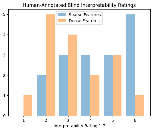
# Let's get the mean and standard deviation of these ratings through a Pandas summary.
# We'll also do a t-test to see if sparse features are truly more explainable than dense features.
import pandas as pd
from scipy.stats import ttest_ind

display(pd.DataFrame(ratings).describe())

ttest_result = ttest_ind(ratings['sparse'], ratings['dense'])
print(f"t-stat: {ttest_result.statistic:.4f}, pvalue: {ttest_result.pvalue:.4f}")
| sparse | dense | |
|---|---|---|
| count | 16.000000 | 16.000000 |
| mean | 4.437500 | 3.250000 |
| std | 1.547848 | 1.437591 |
| min | 2.000000 | 1.000000 |
| 25% | 3.000000 | 2.000000 |
| 50% | 4.500000 | 3.000000 |
| 75% | 6.000000 | 4.250000 |
| max | 7.000000 | 6.000000 |
t-stat: 2.2486, pvalue: 0.0320
Assessment of Results
We can see that some features correspond to the background color of the images (because that was useful when the model was trained to disambiguate between images). We also see that some features correspond specifically to women with blond hair, or images of celebrities in front of specifically dark / specifically light backgrounds. Some neurons are less interpretable and may be combinations of more subtle features discovered during the disambiguation step.
Overall, this analysis provides insight into the types of images that neural networks perceive as similar to each other, and what components each feature vector is made of.
The sparse autoencoder is a lightweight and useful way to uncover monosemantic features, as backed by a t-test. This is simply based on the incorporation of an L1-loss on the sparse feature set.
Ignore
This is me verifying that the ImageDataset loaded images in alphabetical order, for reproducibility after closing this notebook.
visualize_4x4([dataset[267][0]] * 16)
/usr/local/lib/python3.10/dist-packages/torchvision/transforms/functional.py:1603: UserWarning: The default value of the antialias parameter of all the resizing transforms (Resize(), RandomResizedCrop(), etc.) will change from None to True in v0.17, in order to be consistent across the PIL and Tensor backends. To suppress this warning, directly pass antialias=True (recommended, future default), antialias=None (current default, which means False for Tensors and True for PIL), or antialias=False (only works on Tensors - PIL will still use antialiasing). This also applies if you are using the inference transforms from the models weights: update the call to weights.transforms(antialias=True).
  warnings.warn(
import PIL.Image
PIL.Image.open("data/img_align_celeba/img_align_celeba/000268.jpg")