Sound Camera
Published:
This is a year-long research project I conducted as a high-school senior at the Thomas Jefferson High School for Science and Technology.
Sound in Augmented Reality
My goal was to create a portable device to visually display which objects were creating sounds, and I accomplished it, measuring the angular accuracy to be within 15 degrees.
Initial Research and Development
I started by researching how humans evolved to locate sounds to find a source of inspiration for a way to develop a computerized algorithm. My main finding was that humans used the time difference of arrival (TDOA) of sounds reaching each ear to synthesize where sounds were coming from. TDOA is based on the fact that sounds travel at a constant speed, which means that the time delay between two microphones’ detection of a sound is proportional to the two microphones’ distance from the sound. My initial plan was to use an array of microphones as “ears” and compare when any given sound arrived at each microphone.
I also gathered an understanding of how sounds are represented to computers as waveforms. Microphones record data by detecting vibrations in the air and converting these continuous sensor values to discrete binary values (such as from 0 to 65535, -32768 to 32767, or 0 to 256.) The microphone captures the current state of vibration of the air as a frame. By putting a lot of these frames together, microphones create an image of the wave that reached it. When there’s a sudden sound, there’s a sudden vibration in the air that’s captured by the image of the wave (hereafter referred to as the “waveform”.)
It would have been helpful if I had researched already-existing computerized algorithms for sound localization, because I spent a little over a month trying to apply the time difference of arrival concept myself before discovering the widely-used SRP-PHAT algorithm. I recommend that anyone developing an algorithm for their senior research project implement an existing one before trying to design their own.
Time Difference of Arrival
My first attempt at an algorithm was to estimate the time difference of arrival by detecting the time differences between sharp jumps in microphone signals. I used the AV16.3 dataset, which contained recordings of people speaking around an array of eight microphones, to experiment with this algorithm’s potential accuracy. I found out that sharp jumps in a microphone signal can be ambiguous and lead to inconsistent time delays. The following is a sample of a recording from the AV16.3 dataset.
Machine Learning-based Approach
I then tried to create an ML-based algorithm. I found a paper from Amazon’s voice assistant division about how machine learning was used to locate the direction of a user’s voice – they used a convolutional neural network which outputted a “coarse location” where they expected a sound to be vaguely present, and a “fine location” which specified the exact location within that course region. The paper can be found here. I implemented the paper to the best of my ability, but did not have enough data to train with. I tried to simplify the problem by only outputting the coarse location rather than the fine location (which is essentially predicting which microphone detected the sound first.) I achieved a cross-entropy loss of 0.39. Even though it’s better than guessing, it was not particularly accurate.
I realized that I had not verified that the dataset was balanced. I rebalanced the dataset by creating seven identical copies with the sounds being rotated between the microphones. Upon doing this, my loss jumped. This indicated that the previous minor success was due to an imbalanced dataset.
This part of the project taught me to read the training procedure of the paper carefully. I found out that the Amazon paper trained their model on synthetic data and fine-tuned it on AV16.3, rather than only relying on real-life data. This was important because synthetic data allowed them to collect more data than would have been feasible within a short time frame in real life. I recommend looking into synthetic data when training your own models. I spent a lot of time writing boilerplate code that was very specific to the dataset I was using, which resulted in a lot of effort spent on code that was unreusable.
In retrospect, I probably had the time to generate synthetic data and train an accurate ML model, which would have led to some interesting research on the potential of ML for this problem. However, I still found ways to locate sounds effectively that I was able to integrate into my device.
Steered-Response Power Phase Transform (SRP-PHAT)
I still had the AV16.3 dataset code from before, so I decided to test it with a library called ODAS (“Open EmbeddeD Audition System”) (link here). This library was written entirely in C and had significant gaps in its documentation, such as how to customize the audio localization process. To figure out how it worked, I looked at the code itself, and reasoned what parameters I should use with the dataset. I don’t recommend using this library because I later found out that the same functionality can be implemented in Python with ~300 lines of code, and the ability to do sound localization “out of the box” doesn’t outweigh the difficulties in setting it up. The algorithms used by ODAS are an extension of an algorithm called Steered-Response Power Phase Transform (SRP-PHAT) (original paper here).
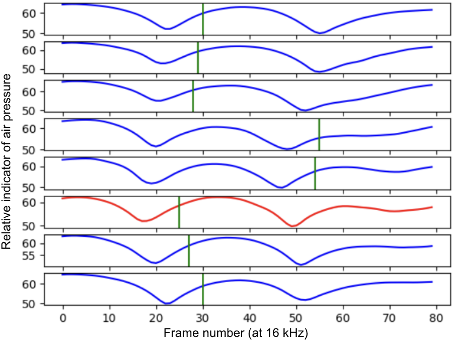
Instead of calculating when each sound arrives and triangulating the location of the source, SRP-PHAT divides space into a grid and calculates how likely a sound was to have arrived from there. Calculating this likelihood is based on the concept of time delay. If, hypothetically, there were a sound at a location, we would know how long it would take to reach each microphone. This is because we choose the location to check, and therefore we know the distance from that position to each of the microphones. The time delay that we would expect is the distance divided by the speed of sound. Therefore, we expect similar features to appear in the audio signals of each microphone at slightly different times.
These two diagrams demonstrate how it works. We set up two microphones at a distance d apart. If we are testing a location to the right of the microphone setup, then we expect the sound to reach the right microphone (d/Speed of Sound) seconds earlier than the sound reaches the left microphone. Therefore, whatever sound occurs at time t = 0 on the right microphone would appear on the left microphone at time t = d/Speed of Sound.
Example of phase offset during SRP-PHAT:
The left microphone’s signal is shifted backward
The black box shows the regions of interest (ROI) for each microphone. We can line up the ROIs by shifting the waveforms from each microphone. Now, we want a way to measure how well the sound from the right microphone matches with the sound in the left microphone signal’s ROI. To measure this correlation, we could consider using cross-correlation.
Cross-correlation takes the average of the product of the intensities between each microphone. Therefore, if both microphones have high intensity or both microphones have low intensity at the same time (i.e., their signals are strongly correlated), the cross-correlation will be high. Cross-correlation works for pairs of microphones, but when we use a microphone array, we will have more than two microphones, and we still want to be able to measure how well the signals between the microphones line up.
This is why we use beamforming instead of cross-correlation. The beamforming algorithm shifts the ROIs of each microphone (a “phase transform”) based on their expected time delays (“steered response power” towards a particular location) and adds them together. This produces a new waveform, which is the sum of several other waveforms. Wherever all the microphones have a high intensity, the intensity of the new waveform will be high. However, if some microphones have high intensity (e.g. 5) and some have low intensity (e.g. -5) then the new waveform will have an intensity that cancels out. Therefore, beamforming allows us to capture the underlying correlation between several microphone signals. The overall quality of a given sound location is calculated by taking the decibel level of the added-together sound. This is the method that ODAS uses for sound localization.
Code to perform beamforming for one grid square xyz:
# For each microphone:
for mic in range(num_waveforms):
   # Calculate the expected time delay
   delay = int(get_time_delay_of_arrival_in_seconds(
       mic_locations[mic], xyz) * sample_rate)

   # If delay < 0, then we should be playing future sounds earlier.
   # If delay > 0, then we should be playing past sounds later.
   # Shift the waveform accordingly, and add to the summed wave.
   if delay < 0:
       summed_waveforms[:-delay] += waveform[mic][delay:]
   else:  # Include delay == 0
       summed_waveforms[delay:] += waveform[mic][:-delay]

average_beam = summed_waveforms / num_waveforms
First, the time delay for each microphone is calculated. Then, the signals from each microphone are shifted by that delay and summed together.
All the components of SRP-PHAT have now been covered. Steered Response Power refers to the act of choosing ROIs that are based on the time delay to each microphone, and the Phase Transform refers to the shifting of the waveforms to make the ROIs line up.
ODAS applies this algorithm over a sparse set of points at a distance of 1 meter from the microphone array, resulting in a hemisphere-like point cloud. The points with the highest intensity have a neighborhood of more precise points sampled. Then, the points in this cloud with the highest intensity are output as JSON.
Making the ODAS configuration work involved writing the geometry of the microphone array used in the AV16.3 dataset to the ODAS config file. To compile ODAS, I needed to install CMake and build ODAS with a few commands: First, creating a “build/” folder, then doing “cd build/”, then initializing CMake with “cmake ..”, and finally building the project with “make install”. This outputted two binary files: “odaslive” and “odasserver.” I only used odaslive, which is a command-line program which could take a config file, read sound data from an audio file, and print the sound locations to standard output or write them to a TCP connection (a socket.) These sound locations are written as JSON objects separated by newlines. In order to compile ODAS, I used the Windows Subsystem for Linux (which simulates Linux on the Windows filesystem) because ODAS uses some low-level functions specific to the Linux operating system. I was also unable to recompile ODAS when I upgraded my Windows computer to a Macbook, because some libraries were not yet supported by Apple’s new chip architecture. I elaborate more on this later, but the result was that I needed to recreate the ODAS library from scratch.
ODAS also came with a visualizer, which required installing Node.js and running the program with “npx electron .” in the directory containing it. The visualizer showed that for the AV16.3 dataset, audio source location could be located along a single axis, but not further than that. Around this point of my development, the hardware arrived. The GitHub repository for the visualizer can be found at https://github.com/introlab/odas_web.
Hardware
I wanted to experiment with real data, so I found the MATRIX Voice microphone array board. I submitted a hardware order on October 12, and it arrived on November 3. I would highly recommend submitting hardware orders earlier than this.
When the MATRIX board finally arrived, I connected it to a Raspberry Pi. Reading any data of any kind did not work. I followed official demonstrations from their website, using the same Raspberry Pi version (v3) and running the same code, but no recordings had any audio features. The board also came with thermometers and accelerometers, and the data from those was “0.” It did not seem to be a problem with the board’s connectivity, because writing data to the board’s built-in LEDs worked.
I tried using other utilities like arecord (a command line tool) and Audacity to record audio data, but none of them were able to detect the board. I factory-reset the Pi and repeated the same process without success. I also purchased another MATRIX board and followed the same steps, along with a factory reset, but was unable to read any data. I considered purchasing another microphone array, so I submitted a hardware order for the ReSpeaker 6-mic circular array kit.
Because my goal was to work with real-world data, I wrote a test algorithm with an Arduino in the two weeks it took for the new board to arrive. I set up an oscilloscope in my basement to read data from Arduino microphones and compare the signals. I used a speaker to play sounds from several locations and exported the recorded signals from the oscilloscope to process them on my computer. The algorithm in this test was to calculate the expected time delay for each microphone and use the cross-correlation between pairs of microphones to calculate a relative intensity level. I implemented this in xcorrmap/xcorrmap.py.

The ReSpeaker board was functional, and I could read its data with a library called PyAudio. There were several helpful demos on the ReSpeaker Wiki:
https://wiki.seeedstudio.com/ReSpeaker_6-Mic_Circular_Array_kit_for_Raspberry_Pi.
Both the ReSpeaker and MATRIX Voice boards connected to the Pi through the General-Purpose Input/Output (GPIO) pins. This meant that the array “stacked” on top of the Pi.
I revisited ODAS, the sound localization library from before. Because the configuration files allowed the output format to be a “socket”, I installed ODAS on the Raspberry Pi and had it output sound locations to an ODAS visualizer on the same device. I soon realized, however, that ODAS was not fast enough to run on the Pi in real time. To achieve this, I offloaded the processing to my own computer, which meant I would need to set up a connection over the network.
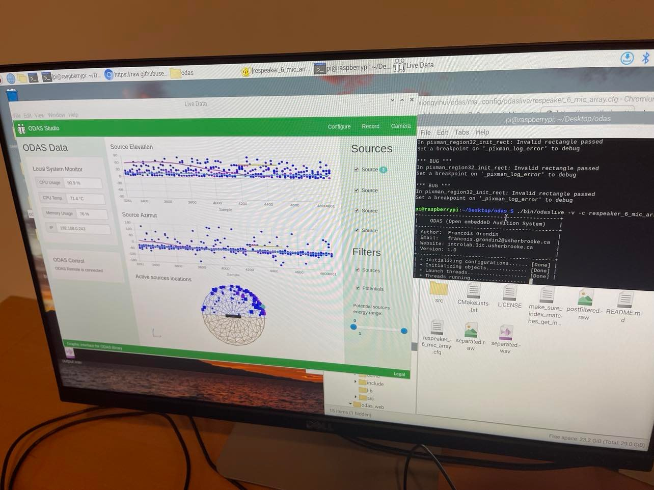
The ODAS visualizer. Each blue dot indicates a high likelihood that a sound is coming from that direction.
Reading Raw Audio Data
I needed a way to record sound data and send it over the network, so I wrote a Python program that read data with PyAudio and established a socket server that I could use to send data to outside servers. This involved creating a TCP server based on the specifications from the Python documentation: https://docs.python.org/3/library/socket.html.
Sending raw sound data required me to learn how sound data is stored. In this case, each “frame” of sound from a single waveform is stored as two bytes: a signed 16-bit integer. There are 8 channels on the ReSpeaker 6-Mic Array, two of which are used for audio playback and can be ignored. When reading from a device with PyAudio, the corresponding waveforms for all channels – whether for recording or playback – are returned. Data is read in chunks, where the parallel streams of data from each channel are serialized in the format “[channel 1 bytes][channel 2 bytes][…][channel 8 bytes]”. The two bytes for each channel store one form of a digitized version of the sound wave. Code for this is in the main() function of vox_server.py.
Sometimes, the channels for the ReSpeaker array would go out of order. Let’s say that the original channel order was (1, 2, 3, 4, 5, 6, 7, 8). Sometimes, the data read under channels (1, 2, 3, 4, 5, 6, 7, 8) would actually be the data corresponding to channels (3, 4, 5, 6, 7, 8, 1, 2), or some other cyclic permutation by 2, 4, or 6 channels. I was able to deal with this because channels 7 and 8 are reserved for playback, so they are always silent when recording audio. At runtime, I would determine which channels had received a sound, and which had remained silent, and shift the order of the channels such that the silent ones were at indexes 7 and 8. After testing (once I had implemented the sound localization algorithm), I found that the order of the input channels was always preserved if the indexes of the output channels were known (channel_permutation.py).
Cloud Data Processing
Once I was able to read and send raw audio data, I needed to be able to consume it on the processing node. Optimally, I would be able to send sound data directly to a server running ODAS, but ODAS had no support for streaming data from a network connection. So, I learned how to use sockets from the Linux documentation and implemented the feature myself. It was very difficult to navigate ODAS’s codebase, as it was written in C, but the knowledge from working with C++ in Computer Vision at TJ transferred well. I made a new kind of sound input called “socket”, which connected to a device given its IP address and inserted the received data into a queue to be further processed. Because this feature integrated with the rest of ODAS, I was able to use the ODAS visualizer to test whether it was receiving the sounds correctly. Fortunately, it was – during testing, the localizations shown in the ODAS visualizer were consistent with where I held a sound source. I now had a way to locate sounds in real time!
Once I verified that this was working, I submitted a pull request to the ODAS GitHub repository. The library authors reviewed the code and approved it. (I was pleasantly surprised that something from this project made it into a real library!)
Visualizing the Data
My overall goal was to create a method to view the indicators in augmented reality, such that indicators would align visually with the objects making the sound. I initially looked at devices that would enable me to create an augmented reality headset with an iPhone by having the screen reflect from a heads-up visor, but I instead prioritized creating a web client because it required less overhead and allowed me to test my algorithm sooner.
Web Client with Reactive 3D Rendering
I first attempted to render the sound locations as 3D indicators in a VR-style environment. I chose to do this because I was comfortable with libraries that I knew I would be able to accomplish this with (React and THREE.js), the web is supported by almost every platform (including mobile phones), and the web is a very convenient way to create user interfaces without significant overhead code. React is a Javascript library that makes dynamic web applications easier to create and less bug-prone by handling all user interface changes behind-the-scenes. It allows the developer to specify the layout of the UI in a syntax that resembles HTML called JSX, which can include dynamic components that automatically respond to changes in the underlying data. I created a React component to render sound locations as spherical indicators in a 3D scene, and I took advantage of the library automatically updating the scene.
However, the direct creation of TCP sockets is not supported by most major web browsers; they only support a protocol called WebSocket. I solved this problem by creating a server that supported both WebSocket and TCP sockets and translated between the two.
Sound data from each microphone was first serialized by PyAudio and sent in chunks to ODAS. ODAS then outputted a list of sound locations to a broadcasting server, which translated them into the WebSocket protocol. Then, they were read by the web client and rendered onto a 3D VR scene by THREE.js and React.
THREE.js includes strong support for virtual reality. When using a mobile device, I was able to control the rotation of the camera based on the orientation of the device with DeviceOrientationControls from an extension of THREE.js called [drei](http://github.com/pmndrs/drei). This enabled me to create a more consistent sense of perspective. I used the library [react-three-fiber](https://github.com/pmndrs/react-three-fiber) to extend React’s dynamic UI support to THREE.js scenes, and allow me to quickly prototype VR environments by using an HTML-like syntax. Each sound location was rendered as a pink sphere, with the opacity being based on the intensity of the sound detected at that location.
<Canvas
    style=
    camera={camera}
    ref={canvasRef}
>
    <Grid />

    <Localizations localizations={localizations.items} />

    <Gate active={mobile}>
        <DeviceOrientationControls camera={camera} />
    </Gate>
    <Gate active={!mobile}>
        <OrbitControls camera={camera} />
    </Gate>

    <pointLight position={[10, 10, 10]} />
    <ambientLight />
</Canvas>
This code sets up a 3D scene in THREE.js
To use `DeviceOrientationControls`, Safari requires the server to provide an SSL certificate. I found it most convenient to use a [CloudFlare tunnel](https://developers.cloudflare.com/cloudflare-one/tutorials/single-command/) at this part of the development stage, because it allowed me to host the server locally and have CloudFlare manage the SSL for me. However, this came at the expense of some of the user experience, because I now needed to type in the IP of the broadcasting server manually.
Algorithmic Improvements
Non-Maximum Suppression
The output from the SRP-PHAT algorithm is a cloud of points, with each point having a corresponding intensity. I performed a threshold to ensure that only points with a relative intensity level above 25% were rendered. While this filtered out random noise, there were still clusters of points where the sound localization algorithm was uncertain of the true maximum location.
To make the localizations look cleaner, I implemented a non-maximum suppression algorithm. This algorithm reduces clusters of points into the member that has the maximum intensity. It is more effective than calculating the overall maximum because it allows for multiple sound sources. This simplification is made by iterating through the points and filtering out points that are not the most intense of the points within a certain Euclidean distance r. Therefore, local maxima are kept in, and all local maxima enforced to be at least r away from each other. The algorithm is computationally inexpensive enough to run in the browser in real time.
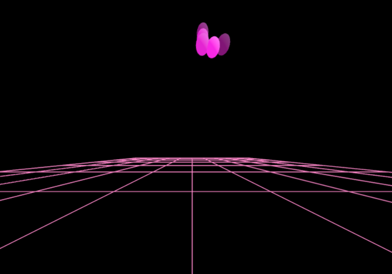 |  |
Before and after applying non-maximum suppression.
The following is a code snippet that performs non-maximum suppression.
def get_non_maximum_suppression_indexes(locations, energies, deduplication_radius):
   unsuppressed_indexes = []

   for index in range(len(locations)):
       location = locations[index]
       energy = energies[index]

       for other_index in range(len(locations)):
           if index == other_index:
               continue

           other_location = locations[other_index]
           other_energy = energies[other_index]

           if _distance(location, other_location) <= deduplication_radius:
               if other_energy > energy or (other_energy == energy and other_index > index):
                   break
       else:
           # Runs if the loop was not broken out of
           unsuppressed_indexes.append(index)

   return unsuppressed_indexes
Frequency-Based Filtering and Ambient Noise Removal
Due to ambient noise in the syslab, high-pitched sounds like my voice would only be detected when they were louder than the fans in the background. To counteract this effect, I created a way to isolate sounds within certain frequency ranges and prevent them from interfering with the detection of other sounds. I converted the waveforms from each microphone into 16 component waveforms, each representing different frequency ranges. For example, one waveform represents all sounds below 125 Hz; the next represents all sounds between 125 Hz and 250 Hz; and so on. Then, I pass these waveforms to the same beamforming algorithm that was used for unfiltered audio.
To create these filtered signals, I modified the “frequency domain” representation of the sound. While sounds can be represented as vibrations in the air as a function of time (the “time domain”), they can also be represented as combinations of several sinusoidal waves at different magnitudes and phases.
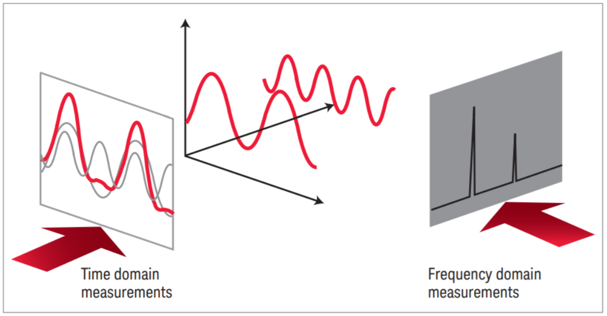
Visual representation of converting between the time domain and frequency domain
Transforming into the frequency domain is done with the Fast Fourier Transform (FFT), and transforming into the time domain is done with the Inverse Fast Fourier Transform (IFFT), both of which can be done with the functions stft and istft from the Python library librosa.
# Create a spectrogram.
# This is done by taking the fft of the last fft_window_length frames, skipping
# fft_hop_length frames between steps.
fft_hop_length = 128
fft_frequency_count = 2048
fft_window_length = fft_frequency_count
# Perform sliding Fourier Transform
spectrogram = librosa.stft(
    waveform,
    n_fft=fft_frequency_count,
    hop_length=fft_hop_length,
    win_length=fft_window_length
)
To isolate sounds within a given frequency range for each microphone’s audio data, I transformed their waveforms into their frequency domain representations, set the magnitudes of the frequencies outside of the desired range to 0, and transformed the sounds back to the time domain.
for bucket_number in range(len(frequency_buckets)):
    # filter_frequencies sets the magnitudes of the frequencies between start_frequency_index and end_frequency_index to 0.
    start_frequency_index = int(
        frequency_buckets[bucket_number][0] * 1025 / 2048)
    end_frequency_index = int(
        frequency_buckets[bucket_number][1] * 1025 / 2048)
    masked_spectrogram = filter_frequencies(
        spectrogram, start_frequency_index, end_frequency_index)

    # Normalize magnitudes to only consider phase offsets of each frequency
    # Not necessary but improves accuracy
    masked_spectrogram_phases = masked_spectrogram / \
        (np.abs(spectrogram) + 0.00001)

    # Reconstructs the time domain signal from the frequency domain signal
    filtered_signal = librosa.istft(
        masked_spectrogram_phases,
        n_fft=fft_frequency_count,
        hop_length=fft_hop_length,
        win_length=fft_window_length
    )
Now that I was able to locate sounds between 0 and 125 Hz, 125 Hz and 250 Hz, and 14 other ranges of frequencies, I could represent sounds differently depending on what their frequency was. First, I could set custom thresholds. I added a step at the beginning of processing that would measure the ambient noise level of each frequency range. Then, the intensity requirement for a sound to be shown on-screen would be calculated based on that. Therefore, frequency ranges with more ambient noise, like 0 to 125 Hz, can be thresholded more strictly than frequency ranges with quieter sounds like a person’s voice. Another benefit was that if there were a high-pitched sound and a low-pitched sound at the same time, they would be more easily isolated and located independently. This is important when a microphone array only has six microphones, compared to the commercial standards of 96 or more.
I chose to replace ODAS by implementing my own version of the SRP-PHAT algorithm in Python (written in test_spectrogram.py). Part of this was inspired by the fact that I had recently upgraded my computer to a new Macbook, and the Macbook had a chip architecture that was unsupported by some libraries that were needed by it. I tried to compile those libraries directly for the architecture, but after a few days of attempts, I found it would be faster to implement it independently. ODAS also only supported one microphone array per process, and I wanted to perform localization on the 16 frequency ranges separately. To integrate this algorithm to my pipeline, I made a Python socket client (vox_client.py) which would connect to the Pi and read a stream of microphone data. Whenever the socket client received microphone data, it would be added to a queue where a separate processing thread would evaluate it. After evaluation, the detected sound locations would be added to another queue, where another thread would send it to the broadcasting server. I divided work into threads because some components used blocking I/O, and the program would become too laggy if it waited for blocking I/O operations to complete before starting to process the most recent sound data.
Evaluation
Upon implementing these improvements, I needed a way to measure the accuracy of the overall algorithm. First, I marked speaker locations at 45-degree increments around the microphone array.
Then, I added a capture option to the web app which would store any sound locations it received to a variable for five seconds before exporting them as a JSON file. Finally, I placed a speaker at each of the locations and captured five seconds of sound localizations from that location. I loaded the sound locations into a post-processing script written in Python, and plotted the sound locations with the matplotlib library. Markers of the same color represent localizations received during the same capture. Each capture was taken with the speaker being at a different location, and they appear to not have significant overlap.
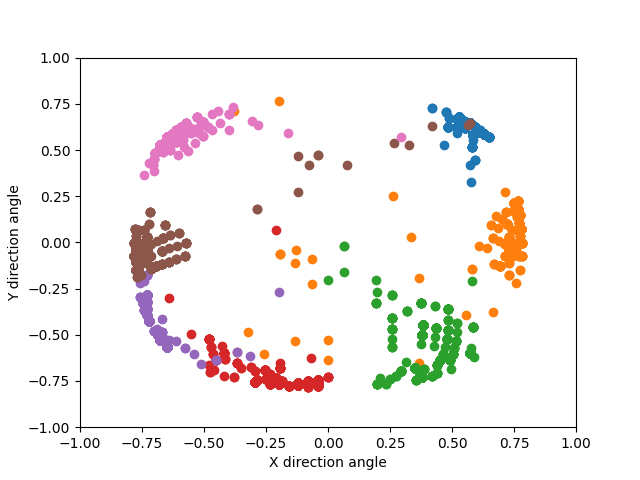
To evaluate these results more rigorously, I took mean and standard deviation of the azimuthal angle (angle around the Z axis) and compared them to the expected angles. I found that the measurements were always within 15 degrees of the true sound source, and that the standard deviations were usually less than 10 degrees.
| Angle (deg.) | Mean | Std. Dev | Mean Absolute Error (deg.) |
| -45 | 312.4 | 4.4 | 3.9 |
| 0 | -2.3 | 19.4 | 7.0 |
| 45 | 56.4 | 9.8 | 12.4 |
| 90 | 101.7 | 8.1 | 11.7 |
| 135 | 149.2 | 8.0 | 14.4 |
| 180 | 177.3 | 11.3 | 5.0 |
| 225 | 222.2 | 6.4 | 5.2 |
Integrating the Camera Feed
Up to this point, I had created a sound “camera” that could locate sounds and render them in a 3D web app. However, the 3D web app lacked a sense of perspective, the locations of sound markers relative to the physical world was subjective. To fix this, I needed to add a visual camera to the back of the device. Unfortunately, because of the difficulty in sending a specific video feed to a web app, I was not able to use the web app I built for this representation. Instead, I created a script that ran locally on the Pi, with the intention that it could be used with an LCD display taped to the front of the device and I could be more efficient by avoiding sending video over the network. I implemented the same algorithms of non-maximum suppression and frequency-based filtering on this new script.
I used an Arducam 5MP Raspberry Pi camera I had at home and taped it to the face of the microphone array. I read from the camera with the picamera Python library and rendered a video feed with OpenCV’s imshow. Then, I set up a socket server to send microphone data to the processing node and read sound localizations. Because I was no longer using neither a web app nor ODAS, I also would no longer need a broadcasting server to translate between the TCP and WebSocket protocol, and my overall processing pipeline was vastly simplified to just a server (the Pi) and a client (the processing node.)
To render the sounds in this new environment, I could no longer use the 3D VR libraries from before, so I represented sounds as circles of varying radius and color, which I drew with OpenCV’s circle function. The color denoted the frequency range, with colors with a deeper blue identifying lower-pitched sounds and colors with a deeper red identifying higher-pitched sounds, and the radius denoted the intensity.
Frequency Range | Color with RGB Value |
0 → 125 Hz | Blue (0, 0, 255) |
125 → 250 Hz | Cyan (0, 255, 255) |
250 → 500 Hz | Green (0, 255, 0) |
500 → 750 Hz | Yellow (255, 255, 0) |
750 → 1 kHz | Orange (255, 127, 0) |
1 kHz → Up | Red (255, 0, 0) |
Sound frequency range vs. Color of indicator
Each sound was tagged with a 3D location satisfying x^2 + y^2 + z^2 = 1; z ≥ 0, and I calculated where to render them in 2D with a perspective projection, setting the plane of the camera at z=-1.
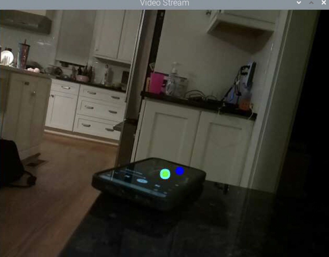 | 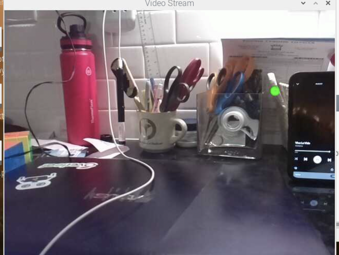 |
Photo of indicators (colored circles) rendered near sound sources.
Because the video feed, networking, and audio streaming were all done from the same program, I split each task into separate threads to ensure that lag from one process didn’t interfere with the others. The server (Raspberry Pi) had the following threads:
- A thread to listen for connections from the processing node
- A thread to read camera data with picamera
- A thread to render annotated camera frames with OpenCV
- A thread to read sound location data from the processing node
- A thread to read sound data with PyAudio and send it to the processing node
Some of these threads, like the thread reading sound location data and the thread rendering sound location data, needed to communicate, and I did this through global variables.
Making It Portable
Making the device portable required (1) removing all dependence on external power, and (2) creating a wireless way to display what was going on on the Pi.
I first submitted a hardware order for a Raspberry Pi Lithium-Polymer (Li-Po) battery chip, which could attach to the opposite side of the Pi from the microphone array. Setting this up simply involved connecting an included Li-Po battery with the regulator chip and using a micro-USB cable to connect the regulator chip to the Pi’s power supply port.
Because all the video rendering was now performed on the Pi, and I did not have an LCD screen to display what was running on the Pi, I needed to render the Pi’s content externally. I submitted a hardware order for a longer HDMI cable, but Dr. Gabor recommended that I look for ways to connect to the device wirelessly. I found out that I can stream data from the Raspberry Pi with the VNC protocol – a standard for screencasting and remote control. I enabled VNC in the Raspberry Pi settings and connected the Pi and my computer to the same Wi-Fi network. Then, I could use the Pi remotely from my computer and project its content during a presentation. This requires knowing the IP address of the Pi beforehand.
Final Device
From top to bottom:
- The Arducam 5MP camera. It is connected to the Pi under the microphone array through a ribbon cable.
- The ReSpeaker 6-mic array. There is a microphone at each corner of this hexagonal chip. It connects to the Pi through the GPIO pins.
- The Raspberry Pi.
- The Lithium-Polymer battery chip.
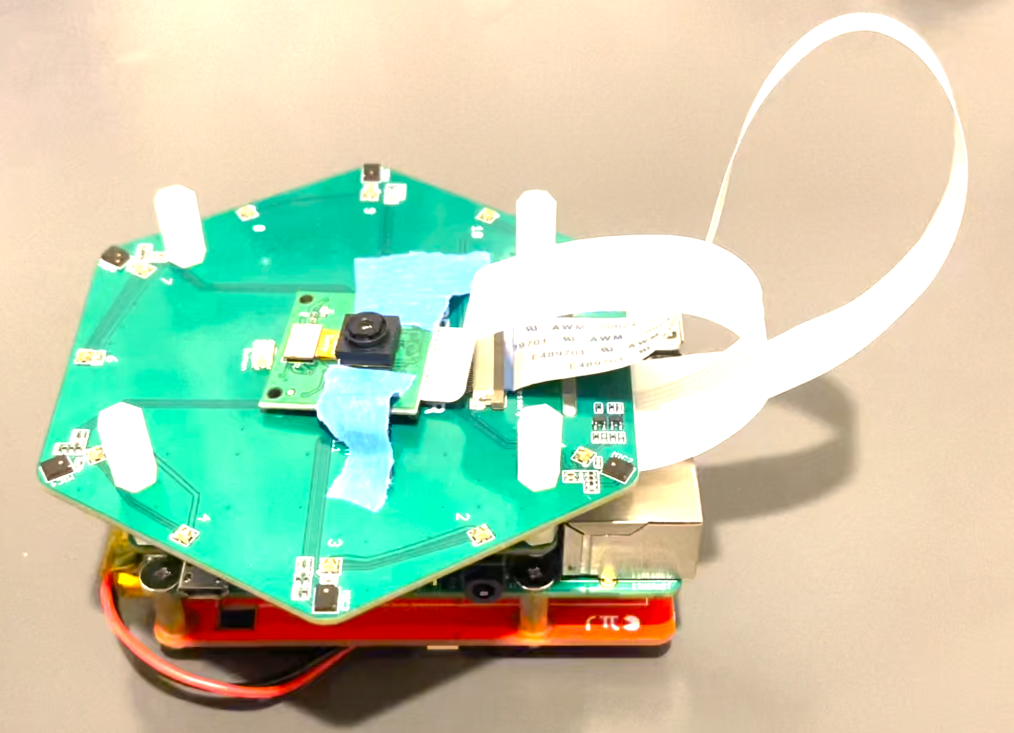 | 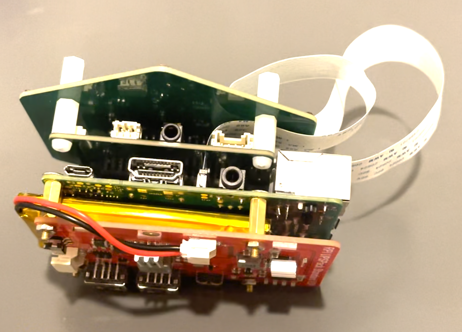 |
It is still a prototype, and while it can’t fit in a pocket, it can easily be used as a handheld device.
Further Directions for Exploration
This project was largely successful, but there are several avenues that I would encourage students in the future to pursue!
- Sound classification. If each detected sound could be annotated with a semantic meaning, maybe with a machine learning algorithm, this could be an interesting project.
- Augmented reality. The current device requires looking at a video feed on a small screen. If the device could be integrated with an augmented reality headset, the sounds would automatically be overlaid with the environment, no camera feed would be needed, and sounds would be significantly more intuitively understood.
- Speech Recognition. This would tie in very well with the augmented reality track: performing speech recognition on separated sounds could enable the creation of live augmented reality subtitles. This could be especially useful for real-time translation applications.
What I Would Have Done Differently
- I could have saved time and conducted research more deeply if I had been more persistent with analyzing the time difference of arrival, machine learning, and beamforming algorithms in the Initial Research and Development phase.
- I would have benefitted from a clearer long-term goal to aid my decisions and prevent myself from spending too much time off-course, such as in Visualizing the Data and I invested a lot of time into a web client with reactive 3D rendering that I did not end up using. Alternatively, I could have looked for a way to send video from the Pi to the web client. Either way, I ended up implementing core functionality twice, and I could have spent this time instead on improving other parts of the project.
Advice for Future Developers
- The Raspberry Pi is a great way to prototype applications that require hardware unavailable on a phone or laptop. However, it comes with a tradeoff of being harder to set up. It will be handy to have backups of both the software and hardware setup on the Pi, and sometimes, the best solution is to factory reset it. The most common method of using a Raspberry Pi is with a keyboard, mouse, and monitor connected over HDMI, but for streaming data from the Raspberry Pi wirelessly, it can be very helpful to investigate VNC software, like VNC Viewer.
- If you’re using Windows, try the Windows Subsystem for Linux (WSL). Linux is much more developer-friendly because of the strong ecosystem of tools and libraries available. Otherwise, you may need to figure out on your own how to compile a given library.