If you have a chessboard, how can you place 8 queens so that none of them are attacking each other? For a board of size N, this is the N-queens problem. We could solve this directly through recursive backtracking; however, I want to see how well we could do with a pure sampling-based approach. Can we treat this “constraint satisfaction” problem as a sampling problem, where the target probability distribution is \(0\) for any boards with attacking queens, and non-zero for “satisfying” boards? For REALLY big boards, sampling-based approaches might be more efficient at finding boards that are nearly optimal.

To solve this problem, I use “rejection sampling”. In a nutshell, this means we have a way to generate “probably good” boards, and then afterwards we filter through those to see which ones are “actually good”. The “probably good” boards form a proposal distribution, and our decision criteria for whether a board is “actually good” is an acceptance ratio.

More mathematically, we have a proposal distribution \(q(y)\), from which we can easily sample and estimate probability densities. Then, using a target distribution \(p(y)\) from which we cannot easily sample but can easily estimate probability densities, we determine whether \(q(y)\) overrepresents a certain sample; if so, by how much; and then reject with a certain probability accordingly. We first sample from the proposal distribution \(y \sim q(y)\), and then \(u \sim \operatorname{Unif}(0, 1)\). Then, we compute \(r = \frac{p(y)}{cq(y)}\), where \(p(y)\) is the target distribution and \(c\) is a constant such that \(r \leq 1\) for all \(y\). If \(u < r\), we accept \(y\) as a sample from \(p(x)\). We can also write this in terms of log probabilities. We have \(\log r = \log p(y) - \log q(y) - \log c\). If \(\log u < \log r\), we accept \(y\) as a sample from \(p(x)\). In this case, because \(\log p(x) = -\infty\) for all \(x\) that don’t satisfy the constraints, we can simply reject any values that do not satisfy the constraints, and accept the values that do.

Rejection Sampling with Uniform Proposal Distribution

We note that no two queens can be in the same row. Therefore, there must be exactly one queen in each row. So, we can represent the board as a list (e.g. \([2, 0, 3, 1]\) for a \(4 \times 4\) board), where the position in the list represents which row the queen is in, and the value at that position represents the column. We can randomly generate such boards uniformly by taking random permutations of \([0, 1, 2, 3]\). To add rejection sampling, we simply check if the resulting board after the random permutation has any attacking queens, and if not, accept it. The proportion of accepted samples to proposal samples is called the acceptance ratio, which I report here.

import numpy as np


def count_conflicts(board):
    has_conflict = [False] * len(board)
    for queen_index in range(len(board)):
        for other_queen_index in range(queen_index + 1, len(board)):
            if board[queen_index] == board[other_queen_index]:
                has_conflict[queen_index] = True
                has_conflict[other_queen_index] = True

            if abs(board[queen_index] - board[other_queen_index]) == abs(
                queen_index - other_queen_index
            ):
                has_conflict[queen_index] = True
                has_conflict[other_queen_index] = True

    return sum(has_conflict)


def is_satisfied(board):
    return count_conflicts(board) == 0


def energy_function(board):
    return np.exp(-count_conflicts(board))


def propose_initial_board_uniform(board_size):
    return np.random.permutation(board_size)

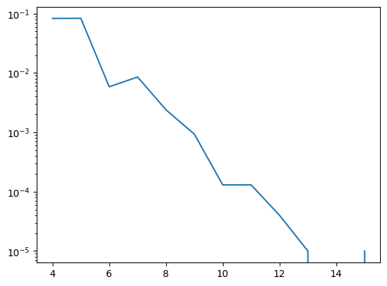
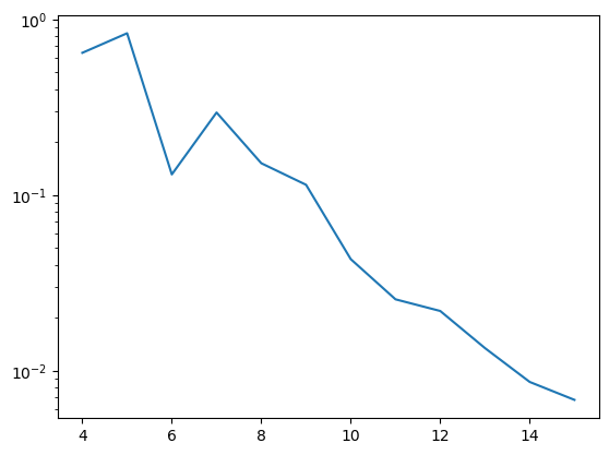
Acceptance Ratio with Increasing Board Size

As we see here, increasing the board size results in an exponentially decreasing acceptance ratio. This suggests that we need to improve the proposal distribution. The better of a match the proposal distribution has, the highest the acceptance ratio. If the proposal distribution matches the target distribution, the acceptance ratio is 1.

X_uniform_proposal = []
y_uniform_proposal = []

for board_size in [4, 5, 6, 7, 8, 9, 10, 11, 12, 13, 14, 15]:
    freqs = {}
    nshots = 100000
    # Now let's sample a couple of boards.
    samples = []
    for _ in range(nshots):
        board = propose_initial_board_uniform(board_size=board_size)
        if is_satisfied(board):
            # for the uniform distribution, E(x) = 0 everywhere, and logc can just be 0, so we can accept all samples.
            samples.append(board)
            board_str = ','.join(str(item) for item in board)
            freqs[board_str] = freqs.get(board_str, 0) + 1

    print(board_size, sum(freqs.values())/nshots, "acceptance ratio")

    X_uniform_proposal.append(board_size)
    y_uniform_proposal.append(sum(freqs.values())/nshots)

import matplotlib.pyplot as plt

plt.plot(X_uniform_proposal, y_uniform_proposal)
plt.yscale("log")
plt.show()

4 0.08289 acceptance ratio
5 0.0831 acceptance ratio
6 0.00584 acceptance ratio
7 0.00854 acceptance ratio
8 0.00239 acceptance ratio
9 0.00093 acceptance ratio
10 0.00013 acceptance ratio
11 0.00013 acceptance ratio
12 4e-05 acceptance ratio
13 1e-05 acceptance ratio
14 0.0 acceptance ratio
15 1e-05 acceptance ratio

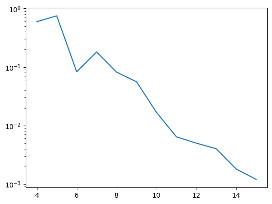
Improving the Proposal Distribution

A nice idea is to use MCMC to sample from a superior proposal distribution, which might represent a sort of “surrogate objective”. For example, reducing the number of conflicts on the board. But wait - how can we do this? Aren’t the distributions unnormalized?

For a simple proposal distribution, we can use the energy function \(E(y) = \operatorname{CountConflicts}(y)\), with the corresponding proposal distribution \(q(y) \propto e^{-E(y)}\). Although we cannot sample from this proposal distribution directly, we can indirectly sample from it using Markov Chain Monte Carlo. There are a few details about Markov Chain Monte Carlo that I will omit here. But the premise is that you take a starting board, \(x_t\), and change it slightly to see if there is a reduction in the number of conflicting queens. If there is, then you accept the change. If there isn’t, then you conditionally accept the change, according to an exponential decay based on the number of mismatched queens. The decision for whether to “accept” the changed board is made with probability \(A(x', x)\), where \(x\) is the source board, and \(x'\) is the changed board. The range of boards you can get by “changing” your current board is called a proposal distribution, \(g(\cdot \\mid x)\).

In the general case, the acceptance function is:

If your proposal distribution is symmetric (proposing a change and proposing “undoing” the change have the same probability for all \(x\) and \(x'\)), then the acceptance function becomes:

This is because \(g(x \mid x') = g(x' \mid x)\) in that case.

Bringing it back to our problem, let’s say that the proposal distribution is a mutation of some sorts. Like switching index \(i\) and index \(j\) of our list representation. There are \(n(n-1)\) ways to make this switch, and each is sampled from uniformly randomly. Therefore, the proposal distribution is symmetric, and we can use the second simplified acceptance ratio.

Now, we wanted to use this to sample from \(q(x) \sim e^{-E(x)}\). Then \(\log A(x', x) = \max(0, \log q(x') - \log q(x)) = \max(0, -(E(x') - E(x)))\). In practical terms, this means we accept any mutation that reduces the number of conflicts, and accept mutations that increase the number of conflicts with exponential hesitancy.

def propose_initial_board_mcmc(E, x0, proposal_distribution, steps):
    # E is the energy function.
    x = [x0]
    for _ in range(steps):
        next = proposal_distribution(x[-1])
        logA = -(E(next) - E(x[-1]))
        if logA >= 0 or np.random.rand() < np.exp(logA):
            x.append(next)
    return x[-1]


def propose_next_board_by_swap(board):
    new_board = board.copy()
    i, j = np.random.choice(len(board), 2, replace=False)
    new_board[i], new_board[j] = new_board[j], new_board[i]
    return new_board

X_mcmc_proposal = []
y_mcmc_proposal = []

for board_size in [4, 5, 6, 7, 8, 9, 10, 11, 12, 13, 14, 15]:
    freqs = {}
    nshots = 5000
    # Now let's sample a couple of boards.
    samples = []
    for _ in range(nshots):
        x0 = propose_initial_board_uniform(board_size=board_size)
        board = propose_initial_board_mcmc(
            count_conflicts,
            x0,
            propose_next_board_by_swap,
            steps=20,
        )
        if is_satisfied(board):
            # for the uniform distribution, E(x) = 0 everywhere, and logc can just be 0, so we can accept all samples.
            samples.append(board)
            board_str = ",".join(str(item) for item in board)
            freqs[board_str] = freqs.get(board_str, 0) + 1

    print(board_size, sum(freqs.values()) / nshots, "acceptance ratio")

    X_mcmc_proposal.append(board_size)
    y_mcmc_proposal.append(sum(freqs.values()) / nshots)

import matplotlib.pyplot as plt

plt.plot(X_mcmc_proposal, y_mcmc_proposal)
plt.yscale("log")
plt.show()

4 0.5934 acceptance ratio
5 0.7486 acceptance ratio
6 0.083 acceptance ratio
7 0.1806 acceptance ratio
8 0.0816 acceptance ratio
9 0.0558 acceptance ratio
10 0.0168 acceptance ratio
11 0.0064 acceptance ratio
12 0.005 acceptance ratio
13 0.004 acceptance ratio
14 0.0018 acceptance ratio
15 0.0012 acceptance ratio

Comparison

It looks like this approach is much better! In both cases, we gave the opportunity for \(100000\) “proposals” or “evaluations”. (For the second, we ran for \(5000\) samples which each took \(20\) Monte Carlo steps to generate). Let’s compare the number of boards we get.

num_boards_mcmc_proposal = [v * 5000 for v in y_mcmc_proposal]
num_boards_uniform_proposal = [v * 100000 for v in y_uniform_proposal]

plt.plot(X_mcmc_proposal, num_boards_mcmc_proposal, label="MCMC")
plt.plot(X_uniform_proposal, num_boards_uniform_proposal, label="Uniform")
plt.yscale("log")
plt.legend()
plt.show()

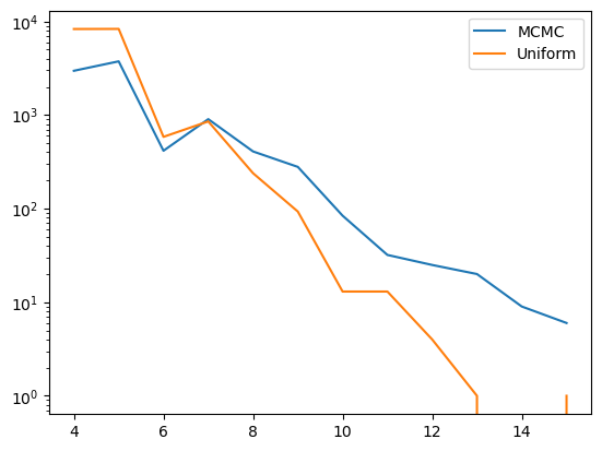
As we can see, using MCMC to initialize drastically reduces the number of samples we need to take. The curve is still exponential (which makes sense, as there are an increasing number of constraints), but the slope has been weakened, allowing us to sample larger boards as if they were a smaller size (here, seemingly as if they were 25% smaller or so). But can we do better? MCMC does not take into account the gradient. Basically, it doesn’t even know that you are better off moving conflicting queens than ones that are already safe. Langevin Dynamics might be a way to fix this. Here, I’m sort of just trying things out and seeing what works.

Continuous Board Representations

It’s possible that my current optimization space is not great. Maybe it’s too easy to get caught in local minima. What if we use a continuous version instead, where we have a tensor \(x \in \mathbb{R}^{n \times n}\)? We can interpret this as \(x_{ij} =\) log probability of the queen in row \(i\) being in column \(j\). Then the energy function can still be the number of conflicts, but we could try to guide each step using the gradient.

Of course, the actual number of conflicts is a discontinuous function of \(x\). We can try to make a continuous approximation, though. The way I’ll try this is by marking the argmax of each row as a “de facto” queen. Then, we can count the number of “expected conflicts” by looking at the squares that this “de facto” queen attacks, and summing up the probabilities. We can see that for the discrete case, this is the same as simply counting the number of pairs of queens that attack each other.

The energy function then becomes the following. Let \(\mathcal{G}\) being the “de facto” queens; i.e. \(\{(i, j) : i \in \{1, \ldots, n\}, j : \forall k \in \{1, \ldots, n\}, k \neq j : x_{ij} > x_{ik} \}\), and let \(\operatorname{Conflicts}(q)\) represent the board squares that a queen at position \(q\) attacks. Let’s let \(\ell(q)\) represent the log probability that a queen is the selected one in its row.

Noting that conflict sets are symmetric; i.e. if \(q_b \in \operatorname{Conflicts}(q_a)\), then \(q_a \in \operatorname{Conflicts}(q_b)\), we can rewrite this as a sum over all of the board squares:

Then, we can calculate the gradient:

This intuitively says that the gradient with respect to logprobs is proportional to the probability of a queen being here times the number of conflicts with argmax queens.

# here, the board is represented by log probabilities.
def continuous_energy_function(board: np.ndarray):
    grad_E = np.zeros_like(board)
    E = 0

    for de_facto_row in range(board.shape[0]):
        # de facto queen
        de_facto_column = np.argmax(board[de_facto_row])
        for j in range(board.shape[0]):
            if de_facto_row == j:
                continue

            # Conflict at row occupied column in row j
            grad_E[j, de_facto_column] += np.exp(board[j, de_facto_column])
            E += np.exp(board[j, de_facto_column])

            # Conflict at diagonal locations
            occupied_column_offset = abs(de_facto_row - j)
            if de_facto_column - occupied_column_offset >= 0:
                grad_E[j, de_facto_column - occupied_column_offset] += np.exp(
                    board[j, de_facto_column - occupied_column_offset]
                )
                E += np.exp(board[j, de_facto_column - occupied_column_offset])

            if de_facto_column + occupied_column_offset < board.shape[1]:
                grad_E[j, de_facto_column + occupied_column_offset] += np.exp(
                    board[j, de_facto_column + occupied_column_offset]
                )
                E += np.exp(board[j, de_facto_column + occupied_column_offset])

    return E, grad_E

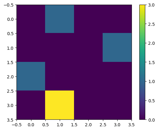
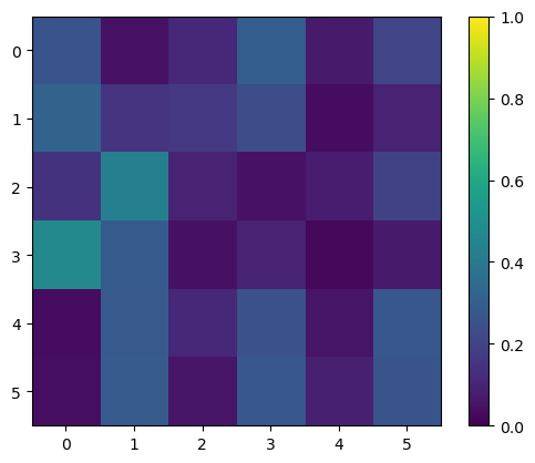
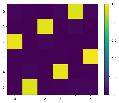
Sanity-Checking our Energy function

Let’s make a simple board with 4 queens, and visualize the gradient of the energy function. We’ll intentionally misplace one of the queens, and plot the gradient of the energy function, \(\nabla_x E(x)\). This misplaced queen conflicts with 3 other queens. Each of the other queens has only a single conflict. Therefore, decreasing the probability of the misplaced queen will proportionally decrease the energy 3 times as much as decreasing the probability of any of the other queens.

board = np.array([
    [-100,    0, -100, -100],
    [-100, -100, -100,    0],
    [   0, -100, -100, -100],
    [-100,    0, -100, -100], # misplaced queen.
])

E, grad_E = continuous_energy_function(board)

# plot the gradient of the energy function.

plt.imshow(grad_E)
plt.colorbar()
plt.show()

Projected Gradient Descent for Optimization with Langevin Dynamics

Here, we use the above energy function and corresponding gradient to perform Langevin Dynamics sampling over “good” N-queens boards. Concretely, at each step, we “should” do (see Eq.6 of Yang Song’s blog):

Where \(\epsilon_t\) is a variance schedule. However I empirically found that just using no coefficient of \(\epsilon_t\) led to better results. Additionally, because we are working with log probabilities, we must project to a simplex, as taking arbitrary gradient steps in log space may cause the probabilities to no longer sum to 1.

def project_to_simplex(x):
    sums = np.sum(np.exp(x), axis=1)
    x -= np.log(sums)[:, None]
    return x

def sample_langevin(x0, noise_schedule, differentiable_energy_function):
    x = [x0]
    for noise_level in noise_schedule:
        xnext = project_to_simplex(
            x[-1]
            - differentiable_energy_function(x[-1])[1]
            + np.sqrt(2 * noise_level) * np.random.randn(*x[-1].shape)
        )
        x.append(xnext)

    return x

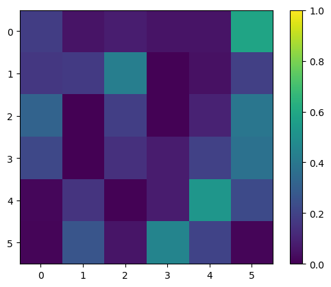
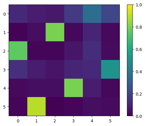
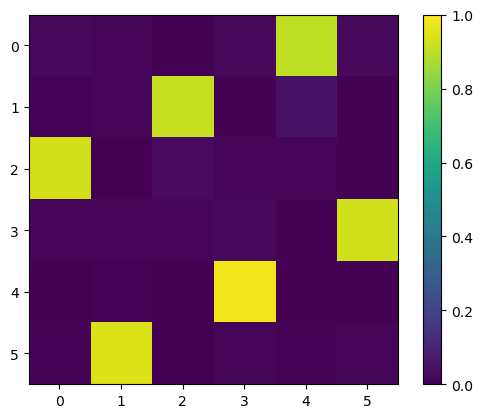
Visualizing an Optimization Path

I had to run this cell a few times to get a nice timeline… So it is not guaranteed. However, we see that it is capable of converging to a valid N-queens board when it gets close enough to the local minimum in the energy function.

nsteps = 100
board_size = 6
steps = sample_langevin(
    project_to_simplex(np.random.randn(board_size, board_size)),
    np.exp(np.linspace(0, np.log(0.001), nsteps + 1)),
    # np.linspace(1, 0.001, nsteps + 1),
    continuous_energy_function,
)
for step in steps[::nsteps//4]:
    plt.imshow(np.exp(step))
    # set value range to 0, 1
    plt.clim(0, 1)
    plt.colorbar()
    plt.show()

Seeing if this results in an even better acceptance ratio

Now, we use Langevin Dynamics to sample from our desired proposal distribution \(q(y) \sim e^{-\operatorname{Conflicts}(y)}\), and see if it creates an improvement over Monte Carlo sampling.

Note that we did forgo the previous prior that all the queens’ columns had to be unique! When we go to check the constraints, before we were guaranteed that each of the queens belonged to different columns. Now, when taking the argmax of each row, we could potentially get two queens in the same column. Is this prior essential?

One of the primary reasons I wanted to create a continuous extension of this problem (beyond the fact that it gives us a sort of gradient) is to allow the proposed samples to “wormhole” through valleys of low density.

def propose_initial_board_langevin(energy_function, nsteps, board_size):
    steps = sample_langevin(
        project_to_simplex(np.random.randn(board_size, board_size)),
        np.exp(np.linspace(0, np.log(0.001), nsteps + 1)),
        # np.linspace(1, 0.001, nsteps + 1),
        energy_function,
    )
    final = steps[-1]

    # plt.imshow(final)
    # plt.show()

    # Convert this to a board with the same representation as before.
    board = []
    for row in final:
        board.append(np.argmax(row))
    
    return board

X_langevin_proposal = []
y_langevin_proposal = []

for board_size in [4, 5, 6, 7, 8, 9, 10, 11, 12, 13, 14, 15]:
    freqs = {}
    nshots = 5000
    # Now let's sample a couple of boards.
    samples = []
    for _ in range(nshots):
        board = propose_initial_board_langevin(
            energy_function=continuous_energy_function, nsteps=20, board_size=board_size
        )
        # print(board)
        if is_satisfied(board):
            # for the uniform distribution, E(x) = 0 everywhere, and logc can just be 0, so we can accept all samples.
            samples.append(board)
            board_str = ",".join(str(item) for item in board)
            freqs[board_str] = freqs.get(board_str, 0) + 1

    print(board_size, sum(freqs.values()) / nshots, "acceptance ratio")

    X_langevin_proposal.append(board_size)
    y_langevin_proposal.append(sum(freqs.values()) / nshots)

import matplotlib.pyplot as plt

plt.plot(X_langevin_proposal, y_langevin_proposal)
plt.yscale("log")
plt.show()

4 0.643 acceptance ratio
5 0.8308 acceptance ratio
6 0.1306 acceptance ratio
7 0.294 acceptance ratio
8 0.1512 acceptance ratio
9 0.114 acceptance ratio
10 0.043 acceptance ratio
11 0.0254 acceptance ratio
12 0.0218 acceptance ratio
13 0.0134 acceptance ratio
14 0.0086 acceptance ratio
15 0.0068 acceptance ratio

Comparison to Other Approaches

The acceptance probabilities seem really great compared to the Monte Carlo version, EVEN without explicitly adding the constraint that all queens belong to different columns. This suggests that continuous representations for optimization could possibly be even more efficient in higher dimensions than discrete counterparts.

Maybe the next thing would be to consider is, how well can we learn a cost function simply from samples? If we trained a model purely with example N-queens solutions, would it be able to infer the cost function?

Perhaps something concerning to note is the runtime. The Langevin approach takes quite a bit longer to run, possibly because we need to take gradient steps on large arrays.

One interesting thing to note is that the gap between the uniform and other approaches increases as the dimensionality of the problem increases.

num_boards_langevin_proposal = [v * 5000 for v in y_langevin_proposal]
num_boards_mcmc_proposal = [v * 5000 for v in y_mcmc_proposal]
num_boards_uniform_proposal = [v * 100000 for v in y_uniform_proposal]

plt.plot(X_langevin_proposal, num_boards_langevin_proposal, label="Langevin")
plt.plot(X_mcmc_proposal, num_boards_mcmc_proposal, label="MCMC")
plt.plot(X_uniform_proposal, num_boards_uniform_proposal, label="Uniform")
plt.yscale("log")
plt.legend()
plt.show()

Closing

Anyway, that’s all I had planned to write for today. It would be interesting to continue exploring whether continuous extensions of discrete problems can allow for better optimization, and more broadly explore the space of Monte Carlo sampling more deeply.